title: Time Series Forecasting with Convolutional Neural Networks - a Look at WaveNet

Note: if you’re interested in learning more and building a simple WaveNet-style CNN time series model yourself using keras, check out the accompanying notebook - ADD LINK that I’ve posted on github. For an introductory look at high-dimensional time series forecasting with neural networks, you can read my previous blog post – ADD LINK.

If you’re reading this blog, it’s likely that you’re familiar with some of the classic applications of convolutional neural networks to tasks like image recognition and text classification. Convolutions are a very natural and powerful tool for capturing spacially invariant patterns. It matters little where in the image whiskers occur when we’re identifying a cat. Similarly, in classifying a document as a court case transcript, the presence of legal jargon phrases matters much more to us than their position in the document. But what about temporal patterns? By a similar token, might there be recurring patterns like weekly cyclicality and certain autocorrelation structures that convolutions are well-suited to model?

The answer is a resounding yes! It turns out that there are specialized convolutional architectures that perform quite well at time series prediction tasks. In this post I’ll discuss one in particular, DeepMind’s WaveNet, which was designed to advance the state of the art for text-to-speech systems. The WaveNet model’s architecture allows it to exploit the efficiencies of convolution layers while simultaneously alleviating the challenge of learning long-term dependencies across a large number of timesteps (1000+). The latter is a frequent pain point for recurrent neural networks, even those that include some long-term memory mechanism like LSTMs.

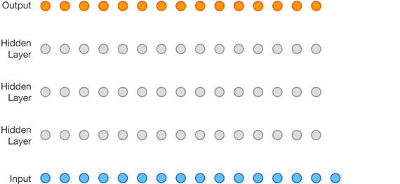
At the heart of WaveNet’s magic is the dilated causal convolution layer, which allows it to properly treat temporal order and handle long-term dependencies without an explosion in model complexity. Here’s a nice visualization of its structure from DeepMind’s post:

The visual is helpful, but let’s try to gain more insight by breaking this down. First of all, what makes a convolution causal? In a traditional 1-dimensional convolution layer, we slide a filter of weights across an input series, sequentially applying it to (usually overlapping) regions of the series. But when we’re using the history of a time series to predict its future, we have to be careful. As we form layers that eventually connect input steps to outputs, we must make sure that inputs do not influence output steps that proceed them in time. Otherwise, we would be using the future to predict the past, so our model would be cheating!

To ensure that we don’t cheat in this way, we adjust our convolution design to explicitly prohibit the future from influencing the past. In other words, we only allow inputs to connect to future time step outputs in a causal structure, as pictured below in a visualization from the WaveNet paper. In practice, this causal 1D structure is easy to implement by shifting traditional convolutional outputs by a number of timesteps.

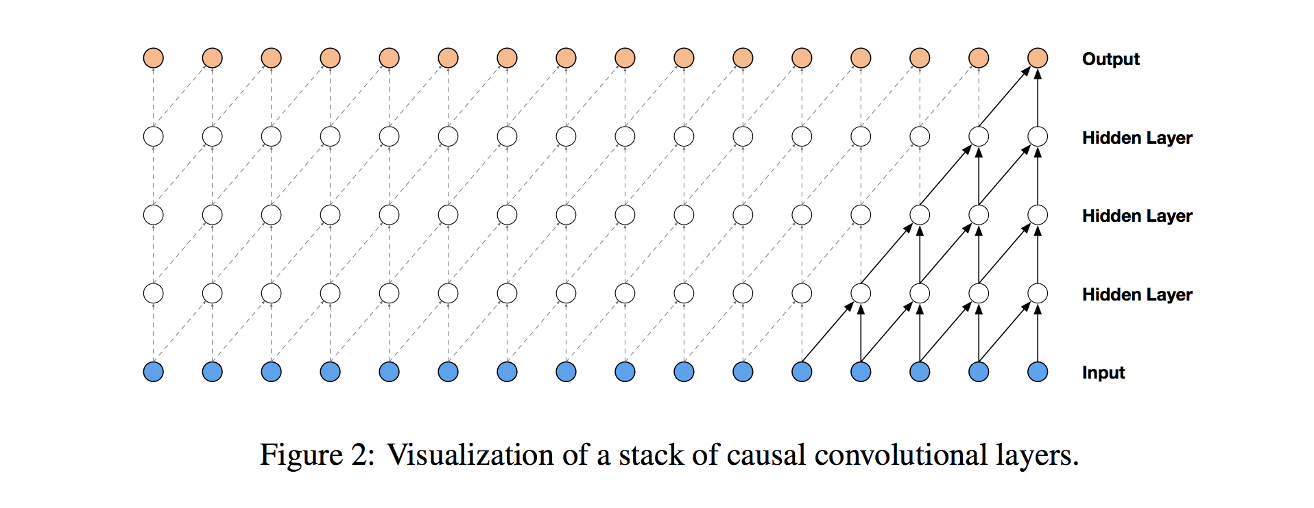
Causal convolutions provide the proper tool for handling temporal flow, but we need an additional modification to properly handle long-term dependencies. In the simple causal convolution figure above, you can see that only the 5 most recent timesteps can influence the highlighted output. In fact, we would require one additional layer per timestep to reach farther back in the series (to use proper terminology, to increase the output’s receptive field). With a time series that has a large number of steps, using simple causal convolutions to learn from the entire history would quickly make a model way too computationally and statistically complex.

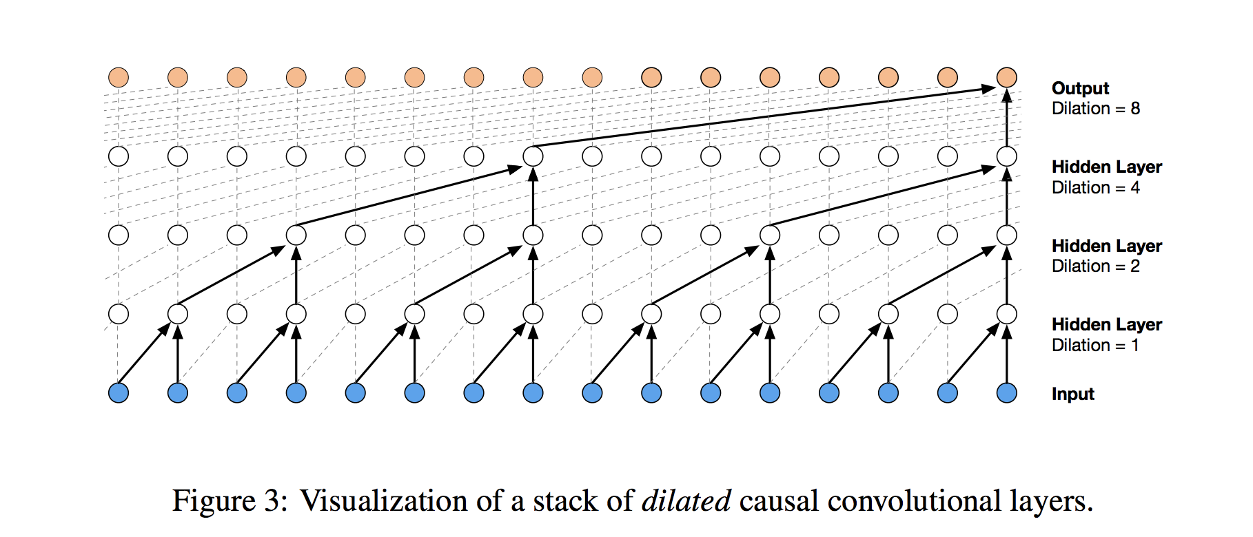
Instead of making that mistake, WaveNet uses dilated convolutions, which allow the receptive field to increase exponentially as a function of the convolution layer depth. In a dilated convolution layer, filters are not applied to inputs in a simple sequential manner, but instead skip a constant dilation rate inputs in between each of the inputs they process, as in the WaveNet diagram below. By increasing the dilation rate multiplicatively at each layer (e.g. 1, 2, 4, 8, …), we can achieve the exponential relationship between layer depth and receptive field size that we desire. In the diagram, you can see how we now only need 4 layers to connect all of the 16 input series values to the highlighted output (say the 17th time step value). By extension, when working with a daily time series, one could capture over a year’s worth of history with only 9 dilated convolution layers of this form.

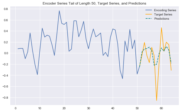
That all sounds great, but how does it work in practice? Using the same wikipedia page traffic data as in my previous post, I trained a bare-bones WaveNet-style network (the code is all in the accompanying notebook). I used a stack of 8 dilated causal convolution layers followed by 2 dense layers. The model trains quickly and does a great job picking up on many recurring patterns across series. The plot below shows an example of future-looking predictions generated by the model. This is the same series as in my previous post on the LSTM architecture, and you can clearly see that these CNN predictions are more expressive and accurate.

This simple CNN leverages the core components of the WaveNet model, but leaves out some additional enhancements that include residual and skip connections and gated activations. Stay tuned for my future posts/notebooks to learn more about these and see the full power of WaveNet. You can also check out the WaveNet paper, or Sean Vasquez’s phenomenal tensorflow implementation of a WaveNet architecture applied to the same wikipedia dataset.