Note: This is an overdue follow-up to my previous blog post introducing the core components of the WaveNet model, a convolutional neural network built for time series forecasting. If you’re interested in learning more and building a full-fledged WaveNet-style model yourself using keras, check out the accompanying notebook that I’ve posted on github.

Picking up where we left off, let’s complete our understanding of the WaveNet architecture by covering the enhancements that it adds around the dilated causal convolutions at the heart of the model. In particular, I’ll discuss gated activations and residual and skip connections, all of which are incorporated into the individual computational blocks that define WaveNet. Although these enhancements aren’t as fundamental to the model as the convolutional structure itself, we need to be comfortable with them to see the full picture. Also, this provides a nice window for exploration into cutting edge techniques that are used as model refinements across a broad range of problem domains including computer vision and NLP.

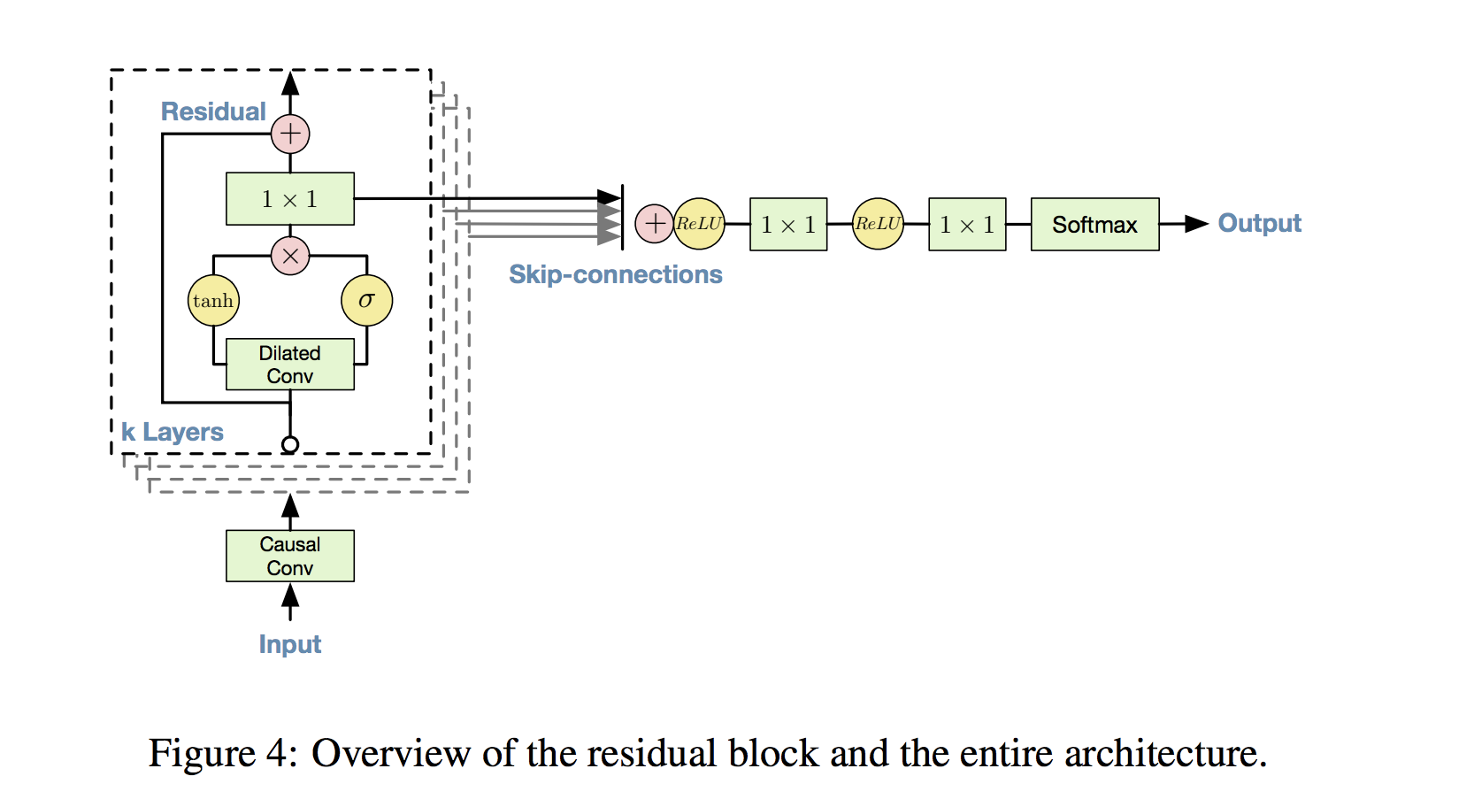
We’ll start by taking a look at a diagram from the WaveNet paper that details how the model’s components fit together block by block into a stack of operations. This way we get an immediate high level view, and have a handy reference as we go for how the methods discussed below are embedded in the model. I encourage you to frequently return to this visual as each component is introduced!

Gated Activations

In the boxed portion of the architecture diagram, you’ll notice that the dilated convolution output splits into two branches that are later recombined via element-wise multiplication. This depicts a gated activation unit, where we interpret the tanh activation branch as a learned filter and the sigmoid activation branch as a learned gate that regulates the information flow from the filter. If this reminds you of the gating mechanisms used in LSTMs or GRUs you’re on point, as those models use the same style of information gating to control adjustments to their cell states.

In mathematical notation, this means we map a convolutional block’s input x to output z via the formula below, where the Ws correspond to (learned) dilated causal convolution weights:

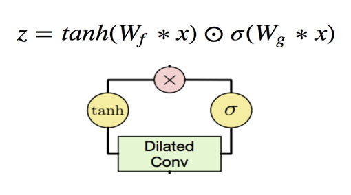
Why use gated activations instead of the more standard ReLU activation? The WaveNet designers found that gated activations saw stronger performance empirically than ReLU activations for audio data, and this outperformance may extend broadly to time series data. Perhaps the sparsity induced by ReLU activations is not as well suited to time series forecasting as it is to other problem domains, or gated activations allow for smoother information (gradient) flow over a many-layered WaveNet architecture.

Residual and Skip Connections

In traditional neural network architectures, a neuron layer takes direct input only from the layer that precedes it, so early layers influence deeper layers via a heirarchy of intermediate computations. In theory, this heirarchy allows the network to properly build up high-level predictive features off of lower-level/raw signals. For example, in image classification problems, neural nets start from raw pixel values, find generic geometric and textural patterns, then combine these generic patterns to construct fine-grained representations of the features that identify specific object types.

But what if lower-level signals are actually immediately useful for prediction, and may be at risk of distortion as they’re passed through a complex heirarchy of computations? We could always simplify the heirarchy by using fewer layers and units, but what if we want the best of both worlds: direct, unfiltered low-level signals and nuanced heirarchical representations? One avenue for addressing this problem is provided by skip connections, which act to preserve earlier feature layer outputs as the network passes forward signals for final prediction processing. To build intuition for why we would want a mix of feature complexities in the forecasting problem domain, consider the wide range of time series drivers - there are strong and direct autoregressive components, moderately more sophisticated trend and seasonality components, and idiosyncratic trajectories that are difficult to spot with the human eye.

To leverage skip connections, a network can simply store the tensor output of each convolutional block in addition to passing it through further blocks. At the end of the block heirarchy, it then has a collection of feature outputs at all levels of the heirarchy, rather than a singular set of maximally complex feature outputs. This collection of outputs is then combined for final processing, typically via concatenation or addition.

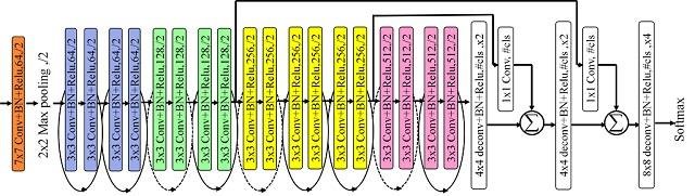
With this in mind, return to the WaveNet block diagram above, and notice how for each block in the stack, the post-convolution gated activations pass through to the set of skip connections. This visualizes the tensor output storage and eventual combination just described. Note that the frequency and structure of skip connections is fully customizable and can be chosen experimentally and via domain expertise - as an example of an alternate skip connection structure, check out this convolutional architecture from a semantic segmentation paper.

Residual connections are closely related to skip connections; in fact, they can be viewed as specialized, short skips further into the network (often just one layer). With residual connections, we think of mapping a network block’s input to output by first passing the input through a learned function, then adding that result to the original input. Traditionally, inputs are just passed to outputs directly via the learned function. The residual connection alternative helps allow for the possibility that the model learns an overall mapping that acts almost as an identity function, with the input passing through nearly unchanged. In the diagram immediately above, such connections are visualized by the rounded arrows grouped with each pair of convolutions. Returning to the WaveNet architecture diagram again, you can see how the residual connection allows each block’s input to bypass the convolution stage, and then adds that input to the convolution output.

Why would this be beneficial? Well, the effectiveness of residual connections is still not fully understood, but a compelling explanation is that they facilitate the use of deeper networks by allowing for more direct gradient flow in backpropagation. It’s often difficult to efficienctly train the early layers of a deep network due to the length of the backpropagation chain, but residual and skip connections create an easier information highway. Intuitively, perhaps you can think of both as mechanisms for guarding against overcomputation and intermediate signal loss. You can check out the ResNet paper that originated the residual connection concept for more discussion and empirical results.

Seeing some results

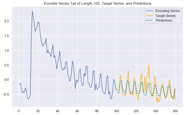
We’ve now worked through all the major components of the WaveNet architecture. With all the time we’ve taken to understand the model, let’s see what it can do! Again using the wikipedia page traffic data, I trained a full-fledged WaveNet-style network to forecast the next 60 days of traffic (the code is all in the accompanying notebook). This time I built a deeper network with a stack of 16 dilated causal convolution blocks that incorporated the gated activations and skip and residual connections discussed in this post. The model takes significantly longer to train than the simpler version, but does a better job picking up on seasonality and trends, adapting to series-specific fluctuation patterns, and handling the longer prediction horizon. The plot below gives one example of future-looking predictions generated by the model, showcasing its successes.

This WaveNet model gets us a long way toward making high quality forecasts on the wikipedia traffic dataset, and so far we’ve only used the raw time series data for training! Why not incorporate relevant exogenous variables like day of the week and language of the page as well to try to make the model even better? We’ll do exactly that in the next update of this series of posts/notebooks, so stay tuned if you’re interested!