The last few months I’ve been working on Porto Seguro’s Safe Driver Prediction Competition, and I’m thrilled to say that I finished in 18th place, snagging my first kaggle gold medal. This was the largest kaggle competition to date with ~5,200 teams competing, slightly more than the Santander Customer Satisfaction Competition. We were tasked with predicting the probability that a driver would file an insurance claim within a year of taking out a policy – a difficult binary classification problem. In this post I’ll describe the problem in more detail, walk through my overarching approach, and highlight some of the most interesting methods I used.

(By the way, if you’re wondering about my team name, it means fear that somewhere in the world, a duck or goose is watching you. Check out those kaggle default duck avatars).

Problem Overview & My Strategy

Seguro provided training and test datasets of close to 600k and 900k records respectively, with 57 features. The latter were anonymized in order to protect the company’s trade secrets, but we were given a bit of information about the nature of each variable. Features related to the individual policyholder, the car they drove, and the region they lived in were flagged as such. All the same, the anonymity limited the role played by feature engineering in my approach. The target variable was quite unbalanced, with only ~4% of policyholders in the training data filing claims within the year (we’ll see that this imbalance plays an important role in my solution). The competition’s evaluation metric was the gini coefficient, a popular measure in the insurance industry which quantifies how well-ranked predicted probabilities are relative to actual class labels. Many data scientists may be more familiar with using ROC AUC for this purpose, and it turns out there’s a simple relationship between them: gini = 2 * AUC - 1. Optimized filing probability rankings are critical for insurance companies, as they help them price individual policies as fairly as possible.

Unsuprisingly, predicting car accidents based on insurance signups is not easy. Even the winning solution to this competition could not break the .65 AUC threshold. Furthermore, the dataset was messy, with large numbers of missing values for some of the most predictive features. In model cross-validation, standard deviations of gini score could be as high as .01, a remarkable level of variance in context (as a reference point, most of the top 40 rankings were decided on the 4th decimal place). These factors made me quickly realize that I’d need to go the extra mile to build a stable model, and that it’d be exceptionally easy to overfit the public leaderboard without a careful methodology.

The strategy I settled on was creating a stacked ensemble, with L2-regularized logistic regression as my meta-learner. Stacking would let me exploit the strengths of multiple different models to decrease generalization error (safety in numbers), and my choice of a conservative meta-learner would smoothly handle prediction multi-collinearities and prevent overfitting. With a final stack of 16 base models, I reached a CV gini of .2924, lowering the standard deviation to .003. The relative stability of my stack was rewarded by a test score quite close to the CV score: .2916.

For those less familiar with stacking, the below diagram taken from this thread neatly visualizes my procedure.

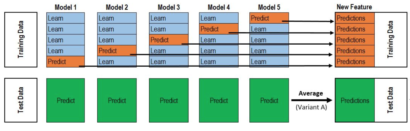
K splits are defined as in K-fold cross validation, with each base model trained once on each of the within-fold datasets for a total of K models. After each training run, out-of-fold predictions are generated and collected alongside test set predictions. The entire collection of out-of-fold predictions then becomes a single feature to be fed to the meta-learner, and the test set predictions are averaged to create a corresponding feature. Running this process for multiple base models, our meta-learner can learn from the training labels how to combine their outputs, and the meta-learner then runs on the test set predictions to generate the final submission output. Since the training data predictions were made out-of-fold, we’re able to simulate our stacker’s performance on data where the labels weren’t known by the base models, as in our test set. For more on stacking, check out this excellent stacking guide.

Stacking works most effectively when the base model predictions are relatively uncorrelated, letting the stacked model minimize their respective weaknesses instead of magnifying them. For this reason, finding a diversity of models to stack is critical. Gains in stacking are often greater with a large number of decent but diverse models than with a smaller number of hyper-tuned strong models. So I made a point of prioritizing model diversity over single model perfectionism, spending more time searching for new models to add to the stack than making optimal adjustments to my existing models. My workflow centered around getting new models up to tolerably good quality, inspecting the spearman correlations between their predictions and my previous base models’ predictions to check for diversity, running cross-validation on the meta-learner, and carefully including only those new models that meaningfully improved CV.

I vetted roughly 40 different models using this procedure, settling on 16 to include in the final stack. I give a complete breakdown of the chosen models in this kaggle post. Most of the models are the usual suspects (gradient boosting with xgboost and lightgbm), but a few are less common methods chosen to add diversity such as regularized greedy forests and field-aware factorization machines. My favorite component of the ensemble was an entity-embedding neural network, which I’ll expand on below. In addition to use of different models, my stack gained diversity through different choices of feature sets - particularly through use of multiple representations of categorical variables (one-hot encoding, target encoding, entity embedding features). Finally, I found an extra diversity edge that secured my high ranking by using a mix of resampling strategies to address the problem’s class imbalance, which I’ll discuss in the final section of this post.

Entity Embedding

At first glance, this dataset seems ill-suited for use of neural networks – it’s a relatively small, tabular dataset with many missing values and a messy, low-signal predictive task. The competition winner blew this assumption out of the water with a groundbreaking neural network approach that centered around denoising auto-encoders, and other top scorers (see here and here) also came up with brilliant NN formulations to include in their ensembles. I didn’t reach their level of sophistication, but I did build a NN that made a key contribution to my stack.

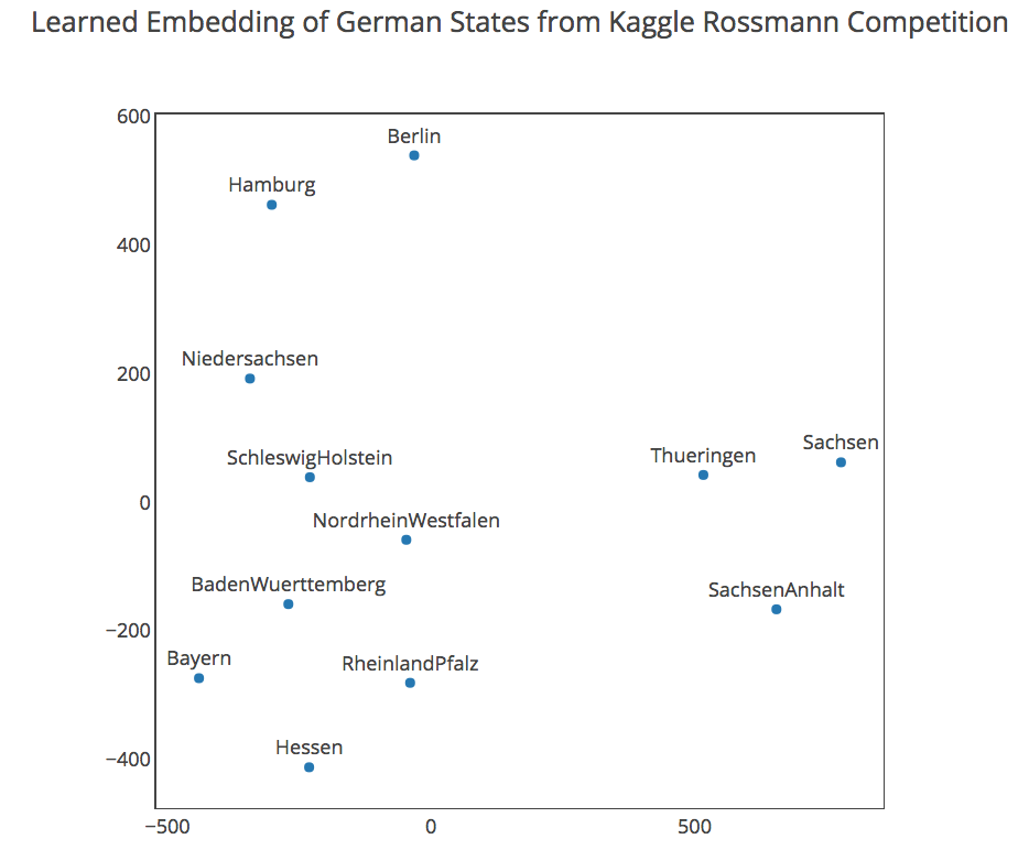
My network was based around an exciting new method for handling high-cardinality categorical variables called entity embedding. This method was well-suited to Seguro’s data, where category counts ran as high as 104 (likely the model of the car). My code for this approach is available here. The core idea behind entity embedding is similar to word embeddings – the goal is to learn a continuous representation of latent qualities that allows us to capture the real meaning of the feature space with reduced dimensionality. With any luck, a representation like this will be handled much better by NN neurons than the naive one-hot-encoding representation with many sparse columns. The chart below from the EE paper gives some intuition behind what EE accomplishes: it shows a 2-dimensional EE representation learned from German states as categories. The learned representation is notably similar to actual German geography!

Formally, EE network architectures add embedding layers for each of the categorical input features – these are fully connected layers that take one-hot-encoded vectors as inputs and have one neuron for each embedding dimension (this dimension is chosen as a hyper-parameter). These embedding layers are then all merged together along with the continuous and binary features, flowing forward into a standard neural network structure. This means that the embeddings are learned via back-propagation, and we can consequently think of EE as a method for supervised dimensionality reduction. In fact, a very neat aspect of the learned embeddings is that they can be reused as features for other models – one of the models in my stack was a lightgbm run on top of entity embedding categorical features, and it provided some diversity gain relative to other boosted models.

I think the broad takeaway from the NN work done on this competition is that with the right level of preparation and structural design, NNs can be competitive with and even outperform the boosting models whose dominance is usually taken for granted on challenging tabular data. Michael Jahrer’s winning solution felt like a paradigm shift for tabular state of the art. I got stuck in a bit of a local optimum with my EE approach, but I have little doubt that I wouldn’t have performed as well without it. That said, my final competitive edge came from going back to the basics to revisit something at the heart of the problem: class imbalance.

Resampling For Model Diversity

There’s some irony in reaching this part last, as I always tell my students that class balance should be the first thing they think about when starting a classification problem. It was clear to me early on that some basic resampling techniques like duplicating the minority class observations (upsampling) within training folds could improve models a bit, but I didn’t realize the full potential of resampling until later. Once I expanded my search for variety beyond different models and features to different resampling techniques, I discovered an untapped source of diversity that pushed my stack over the edge from the top 100 into the top 20.

There are many methods for handling class imbalance. When optimizing for AUC, these methods are used to discourage a model from treating the minority class observations as outliers and ignoring causal signal in the training data. One natural way to accomplish this is by giving extra weight to minority class observations when computing a model’s log loss. Since the minority class then contributes more significantly to the cost function, our model is steered toward paying more attention to how the features cause minority observations. Scikit-learn makes it easy to do this weighting with class_weight parameters (see the logistic regression doc, for example). To obtain balanced class weights, we would find the ratio between majority and minority class counts, assigning a higher weight to the minority class by a factor of that ratio.

As mentioned above, another natural choice is to replicate minority class observations when training in order to emphasize their characteristics and induce better class balance at training time. I used both class weight adjustments (sometimes balanced weights, sometimes more modest adjustments) and upsampling in many of my core models. But yet another option is downsampling, where class balance is shifted by removing observations from the majority class without any manipulation of the minority class. Most commonly, majority class observations are discarded until the classes are balanced. It turns out that this takes a meaningfully different (not better) view of the problem than that of upsampling and class weight adjustments, opening up a new avenue for adding model diversity to the stack. In this case, the difference in view is quantifiable through relatively low spearman correlations (in a world where .95 is low…).

When it comes to the reason for this difference, my belief is that models trained with downsampling can be better at handling probability rankings within the minority class training samples by zooming in on them. Vanilla training or even use of class weights/upsampling focuses on globally ranking observations to separate out classes, figuring out what makes minority samples different enough to merit high probabilities. Downsampling instead lets us work more to figure out how minority samples are different from each other and learn to identify signals of false positivity, all without the distortionary impacts of duplicate samples or exaggerated penalties.

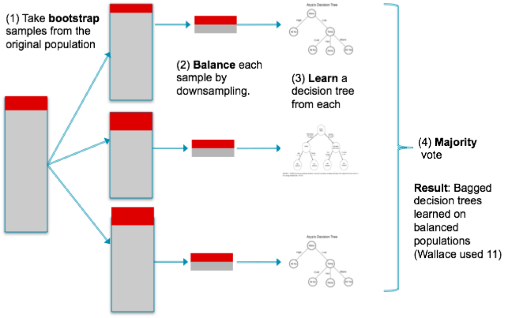
A good question to ask at this point is how one would build downsampling based models that make efficient use of the data. From the above, it sounds like we’re just throwing out a lot of useful data! But we can do better than that using a clever partitioning scheme – let’s call it the downsampling sandwich. First we find the majority:minority ratio (~26 in seguro’s data), then we partition the majority observations in our training data into that many equally sized sets. Instead of training our model one time, we repeatedly train it for each of the majority partitions concatenated with the minority class samples, averaging the results of all of these runs for our final prediction. You can visualize it like this – the minority samples are your sandwich’s protein while the majority samples are the surrounding bread that keeps getting switched out each run. This structure is essentially the same as the “balanced bagging” method, explained well here along with several other interesting resampling techniques.

Extending the sandwich to a 5-fold process for the purpose of stacking, I had to run 26*5 = 130 training iterations for each base model that I wanted to build in this manner. I did this for several base models (xgboost, lightgbm, rgf, ffm) and added them to the stack, seeing my CV gini rise from .291 to .292 (the difference between top 100 and top 20). It was very cool to see this downsampling strategy produce such a significant gain for my stack, validating my original view that finding unusual sources of model diversity would be more fruitful than hyper-optimizing the models I already had.

Conclusions

I learned a lot from this competition, and there’s plenty of extra detail on data processing, treatment of categoricals, and parameter tuning that I did not get into here. I do think I’ve covered the most unique and interesting parts of my workflow. Always be open minded about where diversity can be found when stacking (model, feature, resampling diversity and more!). Perhaps most important, prepare for a world where neural networks work wonders on datasets that you thought they had no right to be remotely competitive on. Seguro’s data may have been an exception to the rule here, but I suspect the more likely outcome is that NN flexibility grows more and more as the theory behind them expands and expertise in designing them deepens.